
Review spectra and chromatograms together in Stacked view, curate individual peptide timepoints, choose your uptake reference, and explore ETD results. These additions join the DIA, PFNet and differential-analysis improvements below.
A complete data-independent acquisition workflow, from building an undeuterated fragment library to reading deuterium uptake off individual fragments.
Import a PFNet model and it sits beside your measured data on the same colour scales, with the residues it could not resolve marked rather than smoothed over.
A volcano plot that applies the accepted hybrid test, so a peptide counts as changed only when the change is both large enough and reproducible enough.
Data-independent acquisition was the single largest piece of work in this period. Fragments do two jobs: they localise a peptide's uptake more finely than the peptide itself, and they show independently when that peptide actually eluted. The second is what removes most of the manual retention time curation from a run, and lets analysis proceed with far less intervention.
Files that need converting to mzML are converted for you. If the required OpenMS tools are not installed, or the data is not actually DIA, the run stops immediately with a dialog that says so rather than quietly producing nothing.
Where Peptide set right-click, DIA DetectA checkbox skips rebuilding the undeuterated library when you already have one, which saves the longest part of a repeat run.
A cross-cell view: the fragment table across the top and a deuteration scatter below it, for spotting which cells in the whole experiment disagree before you go looking at individual spectra.
Where Spectra window, DIA Quality tabSelect a single replicate and you get four stacked panels for it: the precursor chromatogram, one chromatogram per detected fragment shaded by whether the fragment agreed with the others, the labelled fragment spectrum, and the deuteration model fitted through them. A properties sidebar carries the peptide, deuteration and quality numbers.
Where Spectra window, MS2 tab, with exactly one replicate selected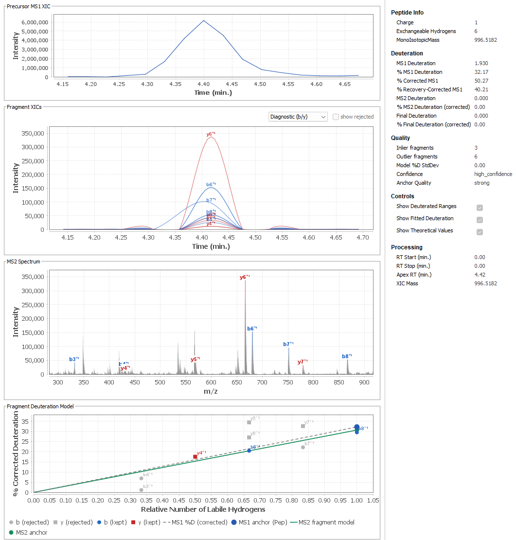
A panel for judging confidence across the run: confidence tiers, counts of cleanly matched fragments, whether the charge states agree with each other, and whether the fragment retention time matched the precursor. It also reports how far the DIA evidence would move each retention window if you let it.
Fragment uptake is fitted as a slope across the fragment series and normalised to the precursor, so a single noisy fragment no longer swings the answer.
Electron-transfer dissociation (ETD) results can be reviewed in sequence coverage, followed one selection at a time, or explored in a separate results browser. The workflow also includes an action to re-run ETD analysis.
View ETD results in the sequence coverage view, so you can inspect them in the context of the protein sequence as part of your analysis.
Where Sequence coverage
The dedicated ETD tab follows the current selection. As you move through the data, it brings the associated ETD results into view for focused inspection.
Where ETD tabA separate ETD All results browser provides a view of the broader set of ETD results. Use it to explore the results beyond the selection shown in the linked ETD tab.
Where ETD All results browserThe ETD workflow includes a re-run action for repeating the analysis when needed, alongside the views used to inspect its results.
Most bad HDX numbers come from measuring the right peptide at the wrong moment. Several features were added specifically to find, check and correct retention windows.
Runs a Sage search over your undeuterated files and updates the peptide set's retention times from the identifications. It offers a dry run first, so you can see what would change before anything is written, and it explains itself and stops if Sage is missing or your files carry no fragment spectra.
Where Protein right-click, Refresh RTs from MS2 (Sage)Where fragment evidence says a peptide elutes somewhere other than the saved window, the correction can be previewed as a table before being applied, and applying it can be rolled back completely.
A window is only corrected when other charge states of the same peptide, or the other replicates of the same cell, agree with the new position. A single outlying measurement cannot drag the window on its own.
Peptide sets are checked against the retention time the peptide was originally identified at, and cells that landed a long way off are flagged for you to look at.
Detection now searches the full declared retention window for the peak apex rather than a narrow slice of it, with score gates so a wider search does not mean a worse pick. Windows that had to be rescued this way are flagged rather than passed off as ordinary picks.
A group of changes aimed at one failure mode: the software confidently reporting deuteration for a peak that is not your peptide.
Detection now checks for a peak sitting just before the peptide's first isotope, for evenly spaced peaks that suggest a different charge state overlapping, and for peptides whose masses conflict with each other. Any of these can veto a pick that would previously have been accepted on score alone.
A parts-per-million ceiling is applied to the combined undeuterated spectrum, so a peak at approximately the right mass is no longer good enough.
The window used to quantify a peptide is capped at the mass it could reach if every exchangeable hydrogen were deuterated. This also fixed a case where the reported centroid could fall outside the very window it was measured in.
Cells that produced nothing on the first pass can be rescued from the combined spectrum, and cells whose signal only appears in a single scan can be latched onto when the evidence supports it. Every rescue is recorded on the cell rather than hidden.
A replicate that was marked usable but produced no measurement used to enter the averages as a placeholder value, quietly pulling means and standard deviations off. Those replicates are now left out and counted separately.
Option H adds a way to rescue on-exchange data, with three categories to distinguish the outcomes.
Where On-exchange rescue, Option HThe cutoff used to accept a fitted signal has been adjusted.
A fix has been proposed to cover a gap in the quality checks for peaks just before the peptide’s first isotope. This item is still proposed.
Support for peptides whose isotope envelope splits into two populations, the signature of EX1 exchange or of two conformations in solution.
A toggle in the spectra view fits two populations to the displayed envelope and draws both, with each one's deuteration, share of the population and how much better the two-population fit is than a single one. You choose which population to assign, and assigning one the data does not support asks you to confirm first.
The assignment is saved with the peptide, appears in the results grid, and is written to the CSV export.
Where Spectra window, bottom bar of the signal view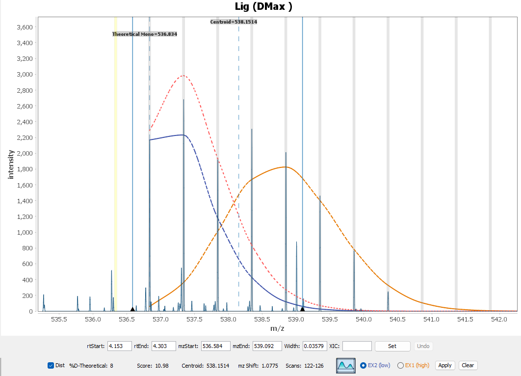
PFNet models exchange at individual residues. HDX Workbench can now bring those results back in and show them next to your measured data.
Import the zipped output and it is filed under the protein. Re-importing replaces that set and leaves any others alongside it, so several models can coexist.
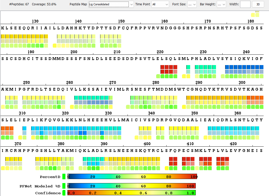
Where PFNet menu, Import PFNet Results (Zip)The coverage dropdown gains a consolidated view per state and a state-versus-control view. Under each stretch of sequence sit three aligned tracks: your measured uptake averaged onto residues, the model's residue-level prediction on the same colour scale, and the model's confidence. Residues the model is least sure of are hatched rather than filled.
Because all three share the sequence ruler, you can see where the model reproduces what you measured, where it departs from it, and whether it was confident when it did. Both views export residue-level CSV files and PyMOL scripts for structure figures.
Per-residue exchange rates or free energies as bars with uncertainty, a track showing which stretches the model could not resolve to single residues, and low-confidence residues greyed so a prediction is never mistaken for a measurement.
Where Spectra window, PFNet tabLu, C., Weber, K. C., McBride, S. K., Reckers, A. & Glasgow, A. A machine learning method for calculating highly localized protein stabilities. Nature Communications 17, 10414 (2026). The paper describes PFNet’s approach to deriving residue-level protein stability from HX-MS data.
Wild type against a point mutant, from one protein entry and one peptide set. The substitution is declared on the wild-type peptide, and both variants are then measured side by side in the same run.
A tagged row is not a mutant row. It defines the wild-type and the mutant candidate together, so there is no second row to add for that peptide and charge. Give the pair a retention window wide enough for both, since a substitution can shift when the peptide elutes.
Where Input peptide set CSV, sequence columnThe number in a tag is a one-based position within that peptide, not a position in the protein or in a PDB file. One protein mutation therefore takes a different number in every peptide that covers it, and each charge state of an affected peptide carries its own tag.
Substitutions are joined inside a single tag with hyphens. AASATAA[MUT-3Y-5P] derives AAYAPAA, with both changes belonging to the same mutant variant rather than describing two separate mutants.
Five columns, with explicit retention-time bounds. The example below carries all three rules at once: both charge states of the tagged peptide are tagged, the second peptide has the position recounted from its own start, and the peptide that does not cover the mutation is left plain.
rt_start,rt_end,charge,sequence,ms score
6.20,6.80,2,AASAA[MUT-3Y],1.0
6.20,6.80,3,AASAA[MUT-3Y],1.0
6.10,6.90,2,GAASAA[MUT-4Y],1.0
8.00,8.60,2,AAAAA,1.0
Retention times are in minutes. Keep the header and the column order, use uppercase one-letter residue codes, and leave no spaces inside a tag. This is an input peptide set rather than a detected-results export, so exported molecular formulas and masses are not something to edit by hand.
Where Saved as a comma-separated .csvIn the Perturbation view the two variants share a comparison row while keeping their own sample observations, so the pair reads as a comparison without hiding what was actually detected in each sample.
Where Perturbation viewIf both variants are marked valid in the same sample at the same timepoint, statistics for that cell are withheld instead of averaging two populations into one number. The detections stay on screen for you to inspect, and an incorrect one should be rejected only after looking at the evidence behind it.
Deciding which differences between two states are real, using the method the field has settled on.
A t-test alone will flag a tiny difference on a very reproducible peptide. A fixed cutoff alone will flag a large difference on a noisy one. The hybrid test requires both at once: the difference must be statistically significant and larger than a threshold calculated from how reproducible your own replicates actually were. Everything else stays on the plot, greyed, with a note saying which of the two gates it failed.
One point per peptide per labelling time, with the size of the difference across the plot and the strength of the evidence up it. Colour says what the point is: protected, deprotected, significant but small, large but noisy, or nothing detectable.
Both cutoff lines can be dragged. Hovering a point gives the full numbers behind it. Clicking one selects that peptide everywhere else in HDX Workbench, so its spectra and uptake curve come up. Dragging a box around a group selects them together for marking or export.
Where Spectra window, Volcano tab, and the Volcano menu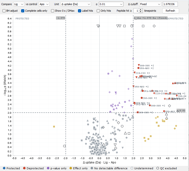
The plot exports as an image, the points or just the hits export as CSV, and a settings snapshot records the comparison, the replicates used, the threshold and how it was calculated, and the software version. The full CSV export gains the same verdict columns.
The sequence coverage map now greys non-significant peptides using the same test as the volcano plot, so two views can no longer disagree about what counts as a change.
A standardised file for HX/MS results, written alongside the usual CSV. It carries the isotope envelope for every measurement, not only the centroid, which is what lets a downstream model work from the peak shape.
Save Report writes a .hxms file for each state into the export folder, next to the CSV and HDXer files. The output is byte-identical to what the PFLink converter returns for the same CSV, so the files can be handed to PFNet or FEATHER without a conversion step in between.
Where Save Report, alongside the CSV exportIllustrative, with the field order the format defines:
METADATA PROTEIN_STATE     apo
METADATA TEMPERATURE(K)   298.15
METADATA pH(READ)         7.00
REMARK   HXMS_DATA_FORMAT v1.0
TITLE_TP INDEX MOD START END REP PTM_ID TIME(Sec) UPTAKE ENVELOPE
TP       1     A   40    44  0   0000   3.0e+01   2.41   0.02,0.11,0.28,0.31,0.19,0.07,0.02
TP       2     A   40    44  0   0000   inf       4.86   0.01,0.06,0.19,0.33,0.26,0.11,0.04
Exported uptake follows the current controls and replicate validity. The fully deuterated control is written with a time of inf rather than a large number, so it cannot be mistaken for a very long labelling point.
The field is filled from the isotope distribution the Workbench already measured, so a residue-level model is not restricted to the centroid and can be run on the peak shape instead. This is what connects the export to PFNet's envelope model.
Every charge state of a cell gets its own record, since charge is not part of a peptide's identity in this format. Discarded replicates and the per-peptide aggregate rows are not exported. The uptake reference can be selected in the Calculations menu and is saved with the experiment.
Modification and mutation tags written in the peptide set become entries in the dictionary at the end of the file, so a downstream reader can resolve what a record refers to without going back to the peptide set.
Exported uptake uses the current controls and replicate validity. When DMax is present, the recovery estimate and deuterium solution concentration header values are written as NA.
When a fully deuterated control is present, HDX Workbench calculates how much deuterium was actually recovered and how much was lost to back-exchange, per peptide, and reports a quality rating for the control itself.
A recovery column in the results grid, so peptides with poor deuterium recovery are visible while you review rather than only in the exported file.
Several runs that used to be left overnight now finish while you wait. The results were checked to be identical before and after each change.
Chromatogram extraction was rewritten to read each file once, over only the retention range actually needed, and to pull all isotope channels in a single pass.
The same windowing applied across the readers, plus opening each raw file once per peptide instead of repeatedly, and searching within spectra rather than scanning every peak.
Statistics are calculated only for the columns you are looking at, the project tree loads a branch when you expand it, and the intensity plots build in the background instead of blocking the window.
One menu item runs the undeuterated detection, writes the peptide set from everything it found, and runs the HDX job from it, reusing the undeuterated results instead of measuring them twice. If any step fails, it cleans up after itself.
Where Protein right-click, Detect + HDX (one pass, reuse 0s results)Each detection run writes a timing breakdown next to the job, so a slow run can be attributed to a stage rather than guessed at.
Switching peptides in the differential view incurs less RAW-data loading overhead, making interactive review more responsive as you move through the results.
Compare multiple measurements in aligned rows, with each mass spectrum beside its extracted ion chromatogram (XIC). Shared axes make it easier to follow changes across timepoints and replicates.
Stacked view keeps the spectra, chromatograms and measurement details together as you work through a selection. Overlay the replicates at each timepoint when you want to compare their signals directly.

The XIC view automatically focuses on the region where the signal reaches at least 10% of the tallest peak, with a one-minute margin on either side. This makes the elution peak easier to inspect.
Where Spectra window, XIC viewUse the ◀ and ▶ arrows beside the width box to narrow or widen charge windows by 5% per click. Your spectrum zoom is preserved while you adjust the window. Width is kept between 0.002 and 90% of the isotope spacing.
Where Spectra view, width boxChoose the reference used to calculate uptake and read mass-unit results consistently across the analysis views.
The Calculations menu lets you use either the measured 0s mean or the theoretical undeuterated-envelope centroid as the uptake reference. The choice is saved with the experiment.
Mass mode displays uptake in Da in the tables, uptake plots, sequence coverage and comparison views. Labels and colour scales follow the selected units.
In consolidated sequence coverage, the percentage-based significance cutoff is converted appropriately for Mass mode. The same numerical percentage is no longer treated as a number of daltons.
When the usual control average is unavailable, calculations fall back to pooled valid 0s and fully deuterated (DMax) controls. If no valid measurements remain in a cell, percentage-deuteration calculations use the qmass reference as a fallback.
Three ways to extend an experiment without reprocessing it: one more peptide, a list of them, or a whole new timepoint. Each reuses the settings the run was made with, and only the new work is searched.
Right-click the HDX job and add the peptide there, so it inherits that job’s working peptide set and the parameters it was run with rather than a fresh set of defaults. The sequence and charge are validated before anything starts, only the added peptide is searched, the results are saved the way a normal run saves them, and the view refreshes so the peptide appears alongside the rest.
Where HDX job right-click, Add peptide(s)The same column-mapping interface the protein editor already uses, so there is nothing new to learn about matching your columns. Sequence and charge are required and retention time is optional. Duplicate and invalid rows are reported rather than dropped quietly, and an import that stopped part way can be resumed from what is left.
Where Add peptide(s), CSV importDrop the raw files into a box for each sample and replicate. The timepoint is registered against the default HDX job’s full peptide set, and only the new files are searched, so the timepoints already measured are left exactly as they were.
Where HDX job right-click, Add timepointExclude a timepoint across all samples and replicates for the selected peptide and charge in the current job. Other peptides retain that timepoint. Restoring it preserves earlier replicate discards, and overall uptake ignores explicitly removed timepoints.
Reversibly exclude a timepoint from the whole experiment while retaining its saved data, then restore it when needed.
Triangle handles on the chromatogram and the spectrum set the window boundaries directly. The text boxes follow as you drag, and pressing Enter afterwards applies the change. The old mass range slider is gone. Zooming still works; the handles only take over while you are actually holding one.
On a multi-cell view the boxes start empty and each cell keeps its own boundary, so you can move one edge across every loaded cell without flattening the other.
To move the whole retention-time or m/z window, drag the bar beneath the boundary handles. Both edges move together, keeping the selected range intact.
Step backward and forward through five levels of Set recalculations, so you can revisit recent edits and restore the fields changed by each recalculation.
Matching the convention used in the field, and the same scale the coverage maps use.
The Marked and Enabled columns are checkboxes you click, instead of a right-click menu, and the change is saved as you go.
Expanded and collapsed branches survive closing and reopening a project, and expanding no longer takes two clicks.
Conversion and search progress is reported instead of the window appearing to hang.
A corrupt result file is skipped with a message rather than breaking the whole load, and there is a repair action that regenerates the affected files.
Sample assignments are validated before the experiment is created, so mistakes surface while you can still fix them easily.
A command-line tool builds experiments from a CSV description, for setting up many experiments at once or scripting a reprocessing run.
Column widths were retuned, the default sort order fixed, and the peptide features column is hidden when nothing populates it.
The left and right XIC arrows shift the retention window using actual scan positions. Coaddition follows the exact scan boundaries, and spectrum zoom stays consistent after edits, Undo and Redo.
FlatLaf is now the default appearance. Detection dialogs have clearer alignment and layouts, including more consistent placement of the Run buttons.
A packaged MSI provides the Windows installation workflow, with improvements to bundled runtime dependencies and installation-directory handling.
The three major vendors are now handled by one common reading layer, which means a feature added for one instrument tends to arrive for the others too.
Bruker folders are recognised throughout the application: in the experiment wizard, when browsing to a folder, in the project tree, and in the spectra views. Ion mobility is taken into account when spectra are combined.
By default the raw data stays where it is and the project keeps a pointer to it, so a large acquisition is not duplicated into the project folder. There is a checkbox if you would rather copy it, and it checks you have the disk space first.
Where Experiment wizard, raw data stepThe vendor detected from your files is shown while you set the experiment up, and a batch that mixes vendors is refused with an explanation instead of failing later in the run.
Lockmass correction is applied when spectra are read, and profile spectra are converted to peaks at the reading boundary rather than later, which removes a source of small mass errors. Detection defaults were retuned for Waters instruments.
Where Detect dialog defaults, and automatically during any Waters runThe instrument's real isolation window boundaries are read out of the raw file instead of being inferred, which matters for assigning fragments in DIA runs.
If a Thermo raw file contains a damaged or unreadable scan, HDX Workbench skips that scan and continues reading the remaining data instead of closing unexpectedly.